Introduction
I have always been interested in image processing since my Computer Science and subsequent employment in document management systems. For my final year project, I failed in the ultimate aim simply because back then there just was not the grunt in the box to keep up with detecting and tracking moving real world objects and process the data quick enough.
That was over 20 years ago and time and hardware have moved on considerably. So as a bucket list idea I wanted to create a motion tracking system.
And fit it out with Fricken’ Lasers.
But, we are moving ahead too quickly. I haven’t even got a machine to run it on yet. Given that it must have Frickin Lasers, I needed an easy way to do signal IO (Input/Output) from a port on the machine. IO boards for PCs were pretty expensive, and given that this is an experimental project I did not want to risk frying my high end monster of a PC by plugging in cheap Chinese crap that I may have wired up wrong in any case.
Hardware
Enter – the Raspberry Pi. Cheap as chips at around 25-30 quid for a 2B+ model, all you need is an SD card and somewhere to plug it in and you are away. They also do video cameras at a low cost, less than 20 quid for a camera and they also do an IR edition of the camera itself – basically the same as what you have in your mobile phone but with the filter missing so it is sensitive to IR spectrum radiation. Handy for a burglar alarm device, that.
There we go, sorted. And as it runs on 5v, you can run it on batteries and put it anywhere you like. Aside from the IO ports, Pi’s also have USB slots so you can plug in keyboards and other peripherals. On board wifi too once you have set it up.
This isn’t an article about the Pi, there are hundreds already written. For a step back into a “proper” computing set up (for tech dinosaurs such as myself) the environment is pretty nifty for 30 quid. It is aimed at the educational and crazy old techie in a shed hobbyist markets and it is quite remarkable what you can do with one.
For around 50 quid I now have my test bed of computer, camera plus a load of free tools to program and test with. Raspberries run a variant of Loonix Linux that is softened a bit for n00bs like myself to make it a bit more out of the box and working than Linux usually is.
All fired up, and ready to go.
Numbers and techie faffing about
The basic algorithm for motion detection is pretty straight forward: connect to a video source and start getting images. Now, a video input is not really continuous, but more a series of quantised data – a single still like a photograph, followed by the next, and the next. These are called frames and they are the basic block of an image stream.
There are countless ways of compressing and expanding these as passing data around is expensive, whether that is just on the motherboard bus or over the internet. You can get what is called a key frame which is the whole frame followed by a series of delta’s that just modify the original picture a little so it looks like the next frame. If the delta gets too expensive to isolate from the picture you have, then just send another key frame (a whole frame), or just have a rule “every 10 frames is a key frame” and not worry about it.
That sort of mucking about is quite unsuited for my purpose– what I want is a series of image stills so I can compare the last frame to the current frame and work out what has changed – this is the “movement” that I need to detect.
Now, computers can only store numbers and they do so in a linear fashion, one number after each other in a line. So in order to be able to do this, we regard an image as a series of dots called pixels. Each pixel – the smallest component part of an image, needs to know what colour and how bright it is so we can turn something that can be stored on a computer into something that can be seen.
There are numerous ways of describing a pixel – and there is always a tradeoff in terms of how to describe it. If we had a simple black and white image, we could say that number 0 is total black, and 255 is total white, and everything in between is a shade of grey, getting lighter as our number gets higher and closer to 255.
That only gives us a limited range of greys though, so how about having more shades? Well, if we had a bigger range of numbers to describe our dot, there would be loads more shades available. Imagine 0 to 65535 as our range – lots more shades of grey to be had and less chance of quantisation where a quite dark dot looks a bit lighter than it should because we only had 256 slots to put it into.
Astute readers will have noticed there are 256 or 65536 total shades in play here – this is because computers use binary bases (on or off) to model numbers. So 28 is 256, 216 is 65536. It just makes it easier for the computer. 28 gives us a total of 8 bits to play with, 216 gives us 16 bits. 8 bits is a byte, 16 bits is a word or two bytes. I always prefer munch to word but that’s techies for you.
The only problem we run into now is that of how much space it takes up. A square image of say 512 by 512 pixels with a range of 256 greys (1 byte, or 8 bits per dot) will need 262144 bytes to store it in. If we up the range to 65536 shades, we have now doubled the image size to 524288 bytes. No problem, eh?
Well, no. At the minute we just have a grey scale pixel description. If we want colour then it gets a bit hairy.
Colour is made up of red, green and blue light, so we could store 3 pixel descriptions for each dot, describing how much of each colour we need to show the right shade. This would be called an RGB https://techterms.com/definition/rgb scheme.
Or we could store Cyan, Magenta, Yellow and Black (CMYK https://techterms.com/definition/cmyk) for easy printing.
Another scheme we could use is YUV https://en.wikipedia.org/wiki/YUV where Y is the luminance (eg grey scale) of a picture and U and V are the differentials to apply. If you read the link previous it has a nice writeup of how television engineers had to find a way to make colour TV broadcasts compatible with black and white signals.
In any case, if we go for an RGB representation for our 512×512 image, we now have to store 3 numbers per pixel. That is 786432 bytes if we are just storing RGB values to a precision of 256 (8 bits or one byte per colour), but we do get quite a lot of colours now. There are 28, or 256 shades for red, green, and blue. 256 x 256 x 256 is 16,777,216 total possible colours which is way more than the human eye can distinguish between (we can see around seven million colours), so 24 bit images are often called “True Colour”.
Anyway, the purpose of all this wittering about bits and bytes and words and stuff is to give you an idea of what the image looks like as far as the computer is concerned. Greyscale images are nice and small by comparison to colour images. We have used an example image size of 512×512 but 1024×1024 will take up 4 times as much space. And when you are processing images, size matters.
We touched briefly on the fact that computers store numbers in binary (ie ON or OFF at the bit level). We can arrange these bits into bytes, which in the time of 8 bit computers were how things were addressed in memory.
Computer memory is contiguous in the way it is addressed in order to load information or save it back. You can imagine a line of boxes stretching from 0 to however big your RAM size is. Depending on the architecture of your computer, each box is capable of storing that many bits. 8 bit computers will store 0-255, 16 bit computers 0-65535 and so on.
But how does this work given that images are rectangular? Limit people to only storing images that are 1 row of dots high but as many as you like sideways?
Nope, we map the x-y space into the linear. Here is a short stream of 8 bit boxes in memory, the index (or address) is the top row, the value in the bottom. Each box can store a number from 0 to 255.
| 1 | 2 | 3 | 4 | 5 | 6 | 7 | 8 | 9 |
| 10 | 127 | 20 | 30 | 255 | 40 | 50 | 127 | 60 |
If our image is 3×3 then we get our greyscale image:
| 10 | 127 | 20 |
| 30 | 255 | 40 |
| 50 | 127 | 60 |
So if we want to know what colour a pixel at row 2 column 3 is then we can calculate the address to fetch that value from as:
((y-1) * w) + x
Where y is the row, x is the column and w is the width of the image. X and Y have their origin at the top left of the image. If you don’t know the width of the image – you’re out of luck. Images usually have at minimum, the dimensions stored as metadata.
This works out nicely so far but we are only looking at greyscale images. If we have RGB images then how do we store that? We could have it as understood we would have the Red block, then the Blue block then the Green, or we could also have it as interleaved RGB where each memory box 1-3 relates to pixel at (0,0), memory boxes 4-6 refer to the pixel at coordinates (1,0) and so on. Either way, we still have to do a lot of faffing about in order to get an arbitrary pixel at (x,y), and that takes CPU time that we don’t have.
If we are using the YUV model of representing our pixels it gets even stranger. For a 4×4 pixel image memory blocks 0-15 will be for the Y component (greyscale), then 16-19 will be the U channel then 20-23 for the V channel. Blending these is a right pain in the arse but is mathematically not too hard. But having to do it over and over takes CPU time. Which we don’t have.
Get. On. With. The. Pretty. Pictures.
It is pretty clear that for image processing, if we can limit the search space (image size) a bit then we are going to help ourselves as we take the load off the CPU. Do we really need colour to do the detection? Nope.
Now here is the dichotomy – we need to have an image that we can analyse, but we also need one to look at. Luckily, the Pi will allow this. The graphics hardware will do all the heavy lifting and even better – we can ask for it in the YUV space so we can ignore everything apart from the Y component, and we handily have our greyscale image. Pi allows a “preview image” to be displayed, and the image stream split off into a converter we can look at the output from, so we can have our cake and eat it. On screen display and a lovely stream of numbers to chew.
Where are my frickin’ lasers?
Insert 70’s style wavy lines as this bit took some time, the documentation for the Pi camera stuff is a little… Distributed, to say the least. The header files for compilation need installing as raw source code instead of nicely packaged libraries, and there’s a bit of faffing about to get things working. Luckily, I did the heavy lifting and you don’t need to hear about it here. Quite often there is a crazy old techie in a shed hobbyist somewhere that has written something and blogs about it. What the research for this project did however was to educate me in how far the internet has fallen – look for “raspberry pi camera code” and you get shedloads of links on where to buy a pi or a camera but precious few links on actual source code. I did find this guy though, who wrote a useful API for the picam stuff: http://robotblogging.blogspot.com/2013/10/an-efficient-and-simple-c-api-for.html where he ripped apart the demo app “raspivid” that comes with the Pi and made it do some new stuff the way he wanted it.
I then had to strip all of the bits of his code that were no use to me and write bits that I needed. Scratching my own itch, so to speak.
Now I have myself in glorious technicolour 1280 by 720 pixels on the screen, and a regularly updated “frame buffer” containing a precious YUV image as a “whole” image rather than a keyframe and a delta. I can casually toss away the U and V parts and there is my big line of numbers that make up a greyscale image.
Then it is on to the algorithm itself. It is basically:
- Get a new picture in an image buffer
- Compare this image to the previous
- Locate the “spikes” of shade which is where the movement is
- Identify the centre of that in co-ordinates.
- Save off the current image as the previous
- Do it all again from step 1.
That’s quite a bit of faffing about and while I was looking for Pi camera source code I accidentally found something called OpenCV https://en.wikipedia.org/wiki/OpenCV which is again some open source Computer Vision stuff. Some kind folks wrote it, some other kind folks packaged it for the Pi and with a simple install command, I have the results of minds immeasurably more powerful than mine at my disposal. And slowly but surely…
Straight out of the box I get a “subtract image” function which lets me do a lot of step 2 for no coding effort. The output is basically ImageNow – ImagePrevious. This gives us an image which is not particularly exciting but shows the movement between the images.
We still have a little further to go though, step 3 of locating the edges of the movement. Luckily OpenCV does that too, with the Erode function which smooths the image leaving just the contour behind. Imagine having a load of sand on a Lego model – the Erode function blows the sand away so you can see more of the shape. Even more fortunately, the library also provides a Canny function which does the edge detection for us! John F Canny (nominative determinism or what?) wrote the algorithm in 1986 and for those like OldTrout who like this kind of thing, there’s a writeup of how it works here: https://docs.opencv.org/2.4/doc/tutorials/imgproc/imgtrans/canny_detector/canny_detector.html
All of this image manipulation and so on is pretty hard to visualise from a stream of numbers so it is just as well that openCV also provides the means to dump our block of numbers out to an image file that we can see. The preview image goes direct to screen so we can’t mess with it.
Around now I added some timings and they were too slow. I reckoned I needed to be able to detect movement at least four times per second to have any chance of the code being usable. My images were just too big, so I had to go back to my code, and change the size of the image I was going to use to faff about with. While still preserving a decent resolution to show on screen. Thankfully, the Pi hardware can be encouraged to do this for you, which I did and then got some much better results than I had been seeing up to now. My direct to screen preview is still at a tasty 1280 x 720 so I can see detail, but the image buffer I want to manipulate is 320×320.
Alright then, at least some pictures then if no frickin’ lasers
So we have our full sized image, at over 160Kb in size:
Resized to 320 x 320 – around 14 Kb in size
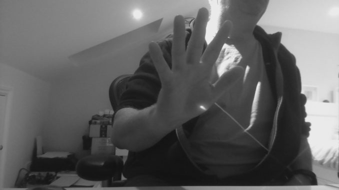
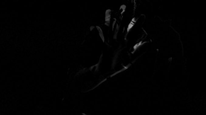
Previous image:
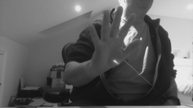
And the current image:

You can see that my hand has moved a little to the left.
We now subtract previous from current so all that remains is “what has changed”:
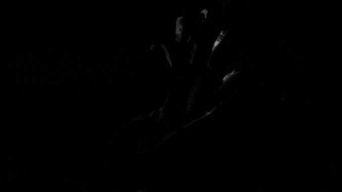
Erode it a bit to get some definition.
And then do the Canny edge detection:
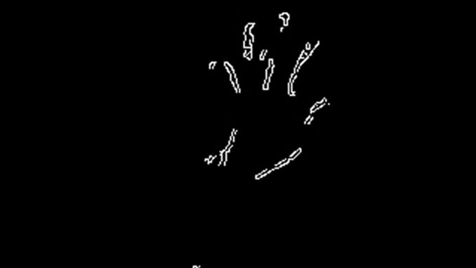
Now we finally have something that is, quite literally, Hitler in black and white. We can easily identify an area on the image where movement is occurring.
And we do, in around 4-5 FPS resolution. The blue rectangle is a handy overlay on the display image, and the crosshair centre is calculated from this. It looks a bit chunky because it is being drawn on a 320×320 canvas and resized to fit into the display resolution of 1280 x 720 for display. That’s a bit of a bugger then, by solving the time taken to process the image we’ve created a problem of scaling.
Right now all of the metrics on what is going on are just being dumped out to file. The Pi has a pretty crap C++ development environment by modern standards and gdb is a powerful debugging tool but there is no point, click and drool inspection of variables, everything is text based. Being an evil capitalist pig running dog, I am used to MicroSoft’s Visual Studio environment, being able to click to set breakpoints in the code and inspect variables for their state. However, this is a behemoth that simply cannot run directly on the Pi. What MS have done though is add a Linux Toolchain capability to Visual Studio – the source is copied across to the Pi, the local compiler is invoked and if your changes are compiled, you will get a runnable program that you can debug. Once again, MS squeezing out the small companies that provide cross compiler chains. But for home use, free.
It is not perfect, the Intellisense is a bit flaky and from time to time it refuses to connect or build. But it is a damn sight quicker and easier for me to see what is going on. Apart from the fact that the preview display writes to video directly, so having a debug session on the PC means the actual display is only visible on the monitor the pi is connected to, it does not appear on the remote desktop window. As I have but one monitor, there was quite an overhead in selecting input1 (pc) then input 2(pi). Luckily, OpenVNC does include the option to broadcast direct from video so that bottleneck was finally overcome.
Lasers. Frickin’ LASERRRS!
The setup is now ready to start acting on the motion detection and at this point I needed a breadboard and a “cobbler” to attach it to the Pi. The Pi IO pins are just 2 rows of pins, easy to get confused which is which so to make it easy, the cobbler bridges from theGeneral Purpose Input Output (GPIO) ports on the Pi to the breadboard. I can then start plugging stuff into a nicely labelled array instead of having to re-solder everything all the time. At the time I had but one servo and a kids toy laser at my disposal, so this is the mark 1 El C Frickin’ Laser Mount.
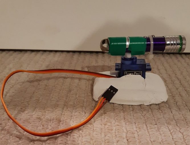
The servo is a 5v model capable of exerting a massive 9 grams of force. The brown cable is neutral, the red live and the orange is signal – should the servo set itself at 0 degrees or at 180 degrees? One complication – the signal is quite sophisticated and needs Pulse Width Modulation https://en.wikipedia.org/wiki/Pulse-width_modulation#Servos. Depending on the uppy-downy-ness of a square wave voltage, the servo will rotate accordingly. Blissfully unaware of this, I had assumed it was voltage driven – 0 volts for 0 degrees, 5v for 180 degrees.
There is however, a whole library that does all of this switching shenanigans for you – the Pi GPIO project, http://abyz.me.uk/rpi/pigpio/ It installs happily and lets you muck about with servos and other outputs to the GPIO pins. The servo would not balance itself when I taped the laser pointer to the servo horn, so I had to nick some of my girl unicorn’s modelling clay to make a stand for it. The switching of the laser is achieved by moving the cable tie collar over the switch for “ON” and then moving it back for off.
Another round of code factoring follows, mostly getting the servo to move when I wanted it to, while the pan and tilt servo gear arrived. And relays. Let’s not forget the relays. Simply switching on and off a laser might not be enough for a burglar alarm, I may want to switch some lights on, release a solenoid holding back the hose pressure or something else, and for that I need 240v and some serious AC amp goodness. Not a piddly 5v 0.5A that might fry the Pi. Relays let me switch mains voltage on and off from a 5v signal.
At this point I realised that the mapping of where the servo thinks it is vs what I see on screen was going to get… interesting. As objects are further away, the angle required to track them is less, and that would get messy very quickly, trying to guess how far away something was based on its size. Instead, I invented a “training mode” where I could fix four points of a rectangle, move the servos to that point and then use that as a guide for where the movement is within the image. The servo’s take an input of 0 for 0 degrees and 255 for 180, all handled nicely through the pigpio interface. Result!
About now, the Pi started to show signs of distress. I was hammering the CPU and starting to bleed a lot of current into the servo and relays, leaving the Pi itself without the energy to keep the screen on. So I had to power the servos and relays from another source, which needed some soldering.
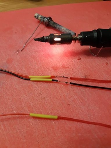
The yellow sleeves are shrink wrap insulation that will be slid over the bare wires and support the joint. This seemed to fix the brownout problem but made the wiring a little messier:
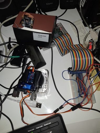
We seem to be getting there. The rainbow cable is feeding the cobbler into the breadboard, and the red and blue lines on the board are now powered separately. The pan and tilt servo is plugged in, and the video camera can be seen mounted in the presentation case of a sawn off cardboard box balanced on top of the Pi. No expense spared, eh?
The servo movement was pretty jerky and making the camera wobble so I used a bit of plastic trunking to make a more stable base. The pan and tilt mechanism is pretty unstable and there was no way of mounting the laser pointer on it without it falling over. A bit of fettling in the shed and we finally arrive at the completed hardware setup.
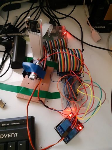
I had thought that mounting the pan and tilt assembly on a bit of hardwood would be enough, but the laser still moved it around. So I had to tape it to the desk to stop it moving. The laser pointer died as I took it apart so I could switch it off and on from the Pi instead of moving the collar, so I bought a 5v laser for less than a fiver off EBay. At the bottom of the picture is the relay unit – two independently controlled SPST relays with common, switched on and switched off outputs. According to the datasheet, you can plug in up to 10 amps at 250 volts. It puts the lotion on its skin or it gets the hose again, indeed.
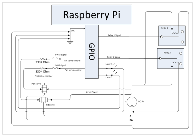
For you electronics nerds, this is what the wiring diagram actually looks like, signal only comes from the Pi and power comes from an external source:
Sweet as, right? We now have motion detection, servos and frickin lasers. Done.
Nope, not yet. We still need to train the servos where to point in relation to the image. So there was a fair amount of coding still to be done – the program now has to run in simple detect mode, detect and track, set a region of interest and two kinds of training so we can find what values the top left and bottom right of the region actually are for the servos.
Here’s a colour picture with FRICKIN LASERS and a few more bits of interest besides. And a spanky home coded heads up display that scrolls up as it updates.
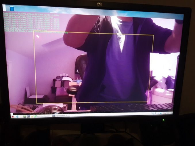
At the top left in green you can see that we are pumping out a healthy >30 frames per second (Video FPS) on the preview, capturing our little 320×320 image (cvVideo FPS) to run detection on at about 30 FPS and still managing to run the detection just under 5 times per second (openCV FPS).
The yellow rectangle is the Region Of Interest (ROI) – if anything moves outside of this we’re not bothered. Just inside the yellow rectangle at the top left, you can see the laser pointer on the sloping ceiling. You can use the keyboard (keys W,A,S,D) to calibrate the pan and tilt servos so the pointer is targeting the top left corner of the rectangle. We can do the same for the bottom right corner and then write the settings for the servo into a config file.
The camera does not move – only the laser pointer does. This is necessary as the ROI rectangle needs to remain a constant so the scalings work. We have 2 scalings to deal with here – the image detection is done on 320×320, the display on 1280×720 and the servos run on a 0-255 scale. The movement centre is based on a (0,0) top left to (320, 320) bottom right coordinate system. We use this to derive a ratio (how far from the top or left edge of the rectangle are we?), and then multiply the servo travel by this amount.
Nice Threads, Man
All of this moving of the servo was pretty jumpy as the camera input is quite sensitive to variations in light levels and shadows once detection thresholds are breached or not reached.. You can see how the blue box in the first video can jump around and that is not good for the servos. So I implemented a background thread that runs alongside the main program, that accepts new coordinates to point the laser to, and if they are too far away from the current position, settles on just moving half that distance for now, has a bit of a rest, then moves the remainder. It also switches the laser on when there is movement detected, then off if there has been no movement for a little while.
Still To Be Done
I think some kind of weighted averaging of the detected centre of movement would be pretty good as the servo does jitter quite badly sometimes.
It’d be nice to put some kind of meta language in place for an if this happens, then do this – like turn on the second laser, activate one or both relays. I could kit up the Pi with some speakers and play some sound “you have fifteen seconds to get the hell out of my back garden” or somesuch. Overall I am pretty chuffed with it so far – would you stay in a garden you should not be in when there is a laser pointer following you around? An unstable optimisation plus a release build of the C++ has seen me get to ~9FPS for the tracking which has really highlighted the need for smoothing the servo movements.
Although a friend did point out that I may need to put some kind of limit as to how long the laser stays on or there will be a pile of dead cats each morning as they cannot leave the chase the laser game that never ends…
© text, images & video El Cnutador 2019
The Goodnight Vienna Audio file