

Dispersive_Prism_Illustration_by_Spigget.jpg: Spiggetderivative work: Cepheiden [CC BY-SA]
Measurements
With linear motion we measured the distance, or displacement (\(\mathbf{s}\)) in metres (\(m\)) as a vector. Which you may recall is a property with both magnitude (its speed) and direction (its heading). When we consider angles we are considering angular displacement.
From school you may remember angles being measured in degrees, 360 of the buggers in a full circle, 90 in a right angle, internal angles of a triangle adding up to 180 and so on. Degrees are actually pretty useful as a unit of measurement, they are easy to understand and easy to work with, nicely dividing into a range of useful angles that can be described without resorting to decimals or fractions.
You may also recall that the relationship between the radius, circumference and area of a circle involves the gad awful constant known as pi, usually shown by the lower case Greek letter of the same name (\(\pi\)). Hence equations such as the one for the circumference (\(C\)) of a circle of a given radius (\(r\)):
\(C=2\pi.r\)
Now using \(\pi\) gets a bit awkward, its easier to leave it as \(\pi\) and express things in terms of multiples of \(\pi\) to avoid having to deal with accuracy issues.
Thus if we have a circle with a radius of say 3 metres, we can describe its circumference in three ways, the first as an actual number: 18.85m (to 2 decimal places), the second in more general terms “nearly nineteen but not quite” or we can describe it as \(3*2\pi\), which simplifies to \(6\pi\) and leave it at that.
When we deal with angles to avoid all of this we can also measure angles in a unit called the Radian, where instead of there being 360 degrees in a circle there are now \(2\pi\) radians in a circle.
Thus 180 degrees = \(\pi\) radians, 90 degrees is \(\frac{1}{2}\pi\) radians and so on. The main benefit being that because \(\pi\) is in the definition of the unit we do not need to put it into the maths and can instead stick with basic numbers
You can do it either way and it all still works, its just that using radians and converting at the end if needed is a lot easier on the brain.
We are now in a position to consider a few new definitions and can then see how the equations we have seen previous can be applied to rotational movement.
Touquing about forces
In the linear world we had the Force \(\mathbf{F}\) which is defined as the mass of the object multiplied by the acceleration, thus \(\mathbf{F}=m\mathbf{a}\).
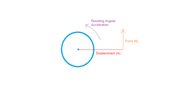
In the rotational world we have Torque, which is a twisting force, this can be visualised to help understand this and how it is defined thus:
Here we have our body and a force acting upon it, but not acting upon the centre of mass but displaced a distance from the centre. If the centre represents a fixed pivot (e.g. an axle) the result of this force will be an angular acceleration as shown.
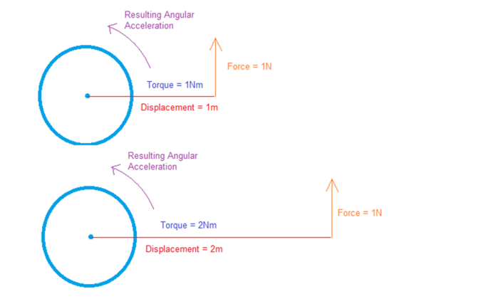
The force applied is measured in Newton metres, defined as a force of \(1N\) applied at a distance of \(1m\). as anyone who has tried to undo a screw or nut that is stuck will know a longer spanner helps, for example the same force applied over two different distances applies a different force thus:
in the linear world the object has a mass m which is defined as the resistance to linear motion, in the rotational world we have angular mass, known as the Moment of Inertia \(I\), which is defined as the resistance to angular motion.
While the actual mass of an object is easy to measure the moment of inertia is less easy (indeed its generally easier to determine it by applying a known force at a known distance and measuring the resulting acceleration). This value depends both on the actual mass of a thing, and the distribution of this mass – for example a disc with a mass of 1kg will have a given moment of inertia if the mass is distributed evenly, and a different one if the mass is concentrated around the rim (like, for example, a flywheel).
We can illustrate this by considering a simple object such as a rigid bar.
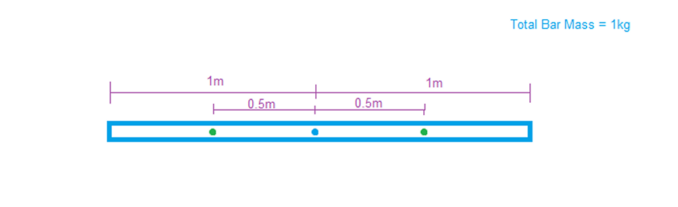
If we assume an even mass distribution, and the centre of mass being the same point as the fixed pivot we can determine the moment of inertia by considering the sum of the mass either side of the pivot.
Each side, again assuming even mass distribution, can be considered as a point mass at its centre, so we have a mass of 0.5kg located at 0.5m from the centre on both sides.
The moment of inertia of each side is \(I = mr^2\), thus \(0.5kg*0.5m^2\) thus \(0.125 kg m^2\) we have two such masses and as such the moment of inertia of the bar is \(0.25 kg m^2\).
Now lets consider the same mass, but distributed differently.
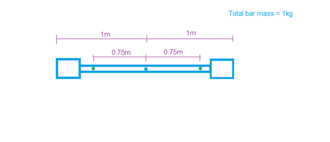
Here we have the same mass, just in a different distribution, the moment of inertia is now \(0.5625 kg m^2\).
The same principle can be applied to other shapes, e.g. circles, by considering the mass on either side of the pivot, if the pivot is in the centre of mass the moment of inertia on each side will balance.
We will consider in future what happens when you change this.
Definitions
Radian: a measurement of an angle, defined as the length of the arc travelled as an object rotates divided by the radius of that arc. As this is a pure ratio (both the length of the arc and radius are measured in metres) there are technically no units, radians are sometimes denoted as “rad” but this is usually left out, e.g. \(2\pi (rad) = 360^o\)
Angular Displacement: a measure of the rotational angle of an object, measured as noted above in Radians. This is usually denoted with the Greek letter \(\theta\) (theta), the initial value is usually denoted as \(\theta_0\) with other subscripts added as required. As with linear motion this is all relative to a frame of reference. This is analogous to displacement (s) in linear motion.
Angular Velocity: a measure of the rate of change of Angular Displacement over time, measured in radians per second (rad \(s^{-1}\)), usually denoted by the Greek letter \(\omega\) (omega). This is analogous to velocity (\(\mathbf{v}\) or \(\mathbf{u}\)) in linear motion. Convention is such that positive angular velocity is clockwise relative to the frame of reference and negative is anti clockwise
Angular Acceleration: a measure of the rate of change of Angular Velocity over time, measured in radians per second per second (rad \(s^{-2}\)), usually denoted by the Greek letter \(\alpha\)α (alpha). One interesting point to note is that unlike linear acceleration where an external force is required, angular acceleration can be induced without an external force by changing the shape of the object (technically changing its mass distribution – e.g. a figure skater changing their speed of rotation by moving their arms).
Torque: the rotational equivalent of a Force, a linear force is a ‘push’ or ‘pull’ effect, Torque is a “twist” effect, clockwise or anti clockwise. The unit of measurement is the Newton metre (Nm)
Moment of Inertia: fundamental property, represents the resistance to angular acceleration. Its value depends upon the physical mass of the object and its shape and mass distribution, it is measured in kilograms metres squared (\(kg m^2\)).
Maffs! (Constant Angular Acceleration)
The five SUVAT equations we have seen previously also apply to constant angular acceleration of a rigid body of a fixed mass around a fixed point (relative to the frame of reference) thus we get the following five equations using the definitions and units noted previously.
\(\omega = \omega_0 + \alpha t\)
\(\theta = \theta_0 + \omega_0 t + \frac{1}{2} \alpha t^2\)
\(\omega = \omega_0 + \frac{1}{2}(\omega_0 + \omega)t\)
\(\omega^2 = \omega_0^2 + 2\alpha(\theta – \theta_0)\)
\(\theta = \theta_0 + \omega t – \frac{1}{2} \alpha t^2\)
the usage of these is essentially the same as before, just in a rotational plane
In the next part we will look at using these equations on our objects and also at ways it is possible to verify these equations, this is slightly more complex than putting a marble on a table, but it is still possible.
© Leopard 2020
The Goodnight Vienna Audio file


